



LCF and HCF fatigue testing of metallic materials
Introduction
ASTM E1829 states that “Fatigue is a permanent, progressive and localized process of structural change in a material subjected to time-varying stress and strain conditions, which can lead to crack formation and/or fracture after a sufficient number of cycles.” Depending on the value of maximum and minimum applied load, the cycle can be distinguished by the value of stress ratio (stress ratio) R (fig.1 – a and b).
When designing, it is useful to know the fatigue behavior of a material, considering that a mechanical component subjected to time-varying loads may exhibit failure even if the average stress level is lower than that corresponding to static failure. With fatigue testing, therefore, one is able to determine how much the material reduces its strength properties when subjected to time-varying loads. It comes to the designer’s aid to determine the S-N curve (better known as the Wöhler curve) and the numerical value of the fatigue limit (fig.2).
Fatigue study can be differentiated according to the number of cycles of interest. For values less than 10^3/10^4 cycles this is referred to as low cycle fatigue ( LCF). For values above 10^4 cycles, high cycle fatigue (HCF) tests are considered. As early as 10^6 cycles, the material may exhibit a horizontal asymptote, called the knee of the curve. In this area, the study is based on determining the fatigue limit.


Low cycle fatigue test (LCF)
In oligocyclic fatigue, i.e., low-cycle fatigue, stresses are affected by loads above the elastic limit of the material. Figure 3 shows the ε-N (strain-life) curve, representative of an overall material response.
Cyclic stresses highlight the plasticity behavior of the material. A typical stress-strain hysteresis cycle (σ-ε) is shown in Figure 4.
Low-cycle behavior is well described by the Manson-Coffin Basquin equation:


With LCF tests, all the coefficients and exponents given above can be determined. LCF tests are performed in strain control. By knowing the tensile strength values of the material, the different strain values to be applied can be defined.
By combining the results of the individual tests, the cyclic (stress-strain) curve of the material can be derived. The latter curve can be compared with the monotonic stress-strain curve and evaluate how cyclic loads can change material properties.
The tests are carried out using a servohydraulic machine (see fig.10).
Deformation is detected by a contact extensometer applied to the specimen (fig. 6). High-temperature testing, up to 1000°C, can be performed using a furnace placed around the specimen (see fig. 11). The specimens used may have different geometry:
- Cylindrical section specimens with cylindrical section or continuous radius
- flat specimens with rectangular cross section


High cycle fatigue test (HCF)
Determination of the S-N curve
One of the most common representations of high-cycle fatigue tests is the S-N (Stress-Life) curve. For the determination of the S-N curve, the standard requires at least 15 specimens to be tested. It is necessary to know in advance the tensile strength values of the material. Only then will it be possible to best define which loads to apply to the fatigue tests. Usually three tests are performed for five load levels. The resulting graph is shown in Figure 7. On the y-axis is graphed the applied stress value expressed as either maximum stress or cycle amplitude. On the x-axis is graphed the value of number of cycles. The maximum number of cycles (runout) for a fatigue test is usually 107 cycles. For ferrous materials the curve, at high cycle numbers, shows a horizontal asymptote. This value represents the fatigue limit value σf. Below this value the material can be considered to have an infinite life, thus not affected by fatigue failure. Nonferrous alloys, on the other hand, do not have a true asymptote, but the curve continues to have a decreasing trend. Tests can be performed on different types of machines. The first system is the vibrophorus, a resonance testing machine that uses a mechanical resonator connected to an electromagnetic drive. Dynamic load is generated by an oscillation system that operates when the system is operating in full resonance. Force is applied by moving the upper crossbeam with the ball screws (fig.8). Tests can also be performed at high temperature, up to 1000°C by employing a furnace placed around the specimen (fig.9). Another type used is a servohydraulic machine (fig.10). Again, it is also possible to perform tests at high temperature (fig.11). These two systems apply the dynamic load in the direction of the specimen axis. The specimens used can have different geometry: cylindrical section specimens with a cylindrical section or continuous radius or flat specimens with a rectangular section. There is the possibility of performing the test by rotating the specimen and applying the load to the ends of the specimen. This mode of testing is possible by employing a rotating bending machine (fig.12 a and b). In this case the specimens used will have a cylindrical cross section.


Determination of fatigue limit
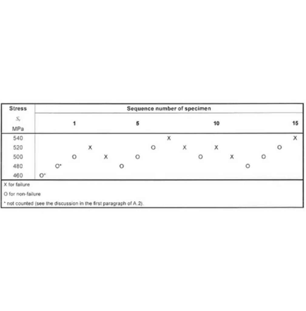
With high-cycle fatigue tests, the fatigue limit value can also be determined. This value is nothing more than the stress value for which the S-N curve reaches the horizontal asymptote, that is, the curve tends to flatten (fig 7). Again, the standard requires at least 15 tests to be performed. The load of the first test is defined by referring to the runout load (load for which there is no failure of the specimen) obtained in the S-N curve. The next test should be carried out at a higher load in case of the achievement of runout without specimen failure.
In the event that the test ends in failure of the specimen, the applied load should be reduced. The load variation between tests is kept constant throughout the activity. Through equations in the standard, it is then possible to derive the fatigue limit value σf.
Do you need a fatigue test?
Request information